AlphaFold Architecture
The AlphaFold system implements several novel techniques to solve the protein structure prediction problem. The main goal of this article is to summarize and highlight novel machine learning practices used, in the form of “Frequently Asked Questions” a machine learning practitioner might ask.
This post refers extensively to the supplementary information article, which provides in-depth descriptions of each component.
Overview
There are two main neural network modules of the AlphaFold system.
- Evoformer (first 42 blocks): jointly refines (1) a pairwise representation of each residue in the sequence, and (2) a multiple-sequence alignment representation of the evolutionarily similar sequences.
- Structure (last 8 blocks): extracts atomic coordinates and angles from the Evoformer representation.
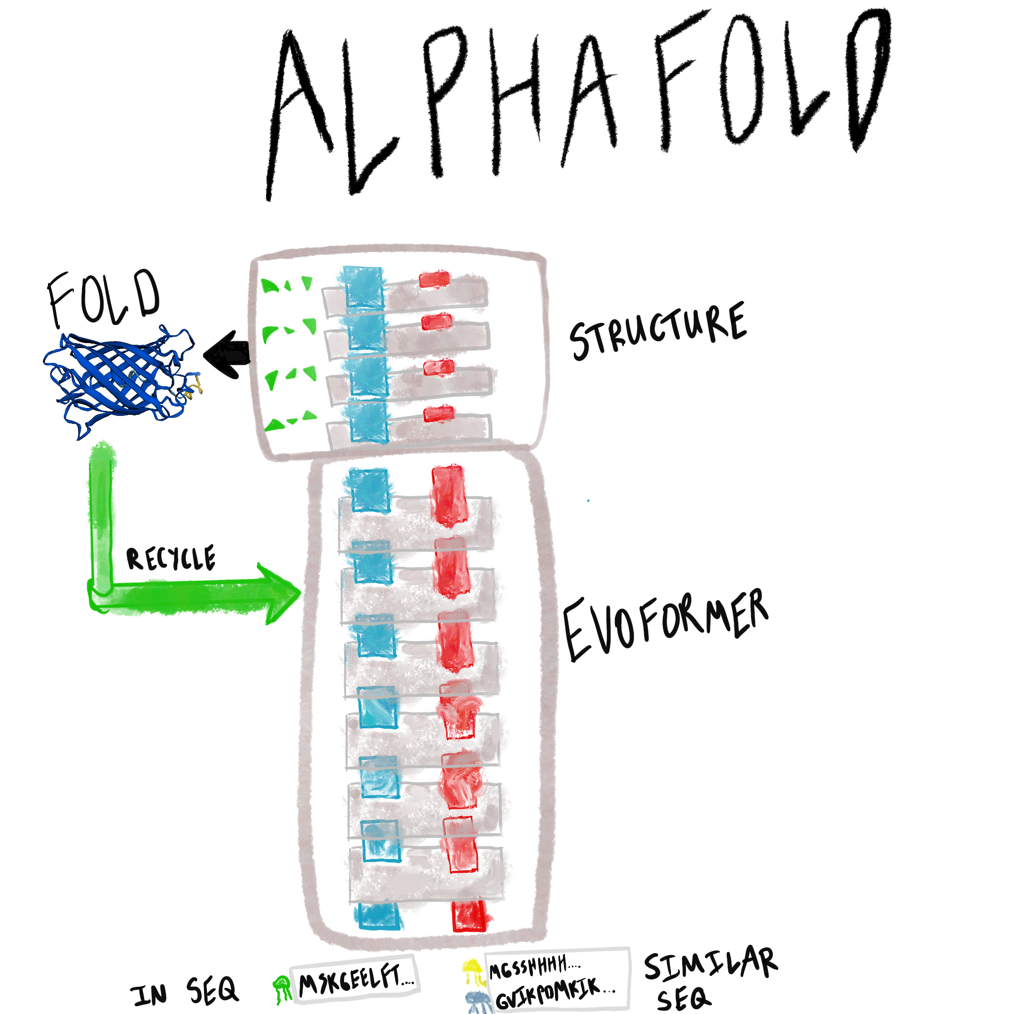
The model is trained end-to-end, and so has a novel architecture designed for information flow and includes several novel loss functions. AlphaFold also introduces the generic concept of recycling neural networks, which was an important component of the model and may become more widespread long-term.
Beyond the architecture, this post also includes some background details about the task, and input msa features, along with some back-of-the-envelope calculations related to the training setup, and inference setup. An overview table now follows:
| Key Detail | Description |
|---|---|
| Inputs | Amino acid sequence; similar sequences (MSA) (see task) |
| Outputs | Protein structure: X,Y,Z of each atom in the amino acid sequence; $\phi$, $\psi$, and other angles. (see task) |
| Quality Metric | Global distance test (% of atoms close to reference), template modeling score, predicted local distance test. (see task and quality metrics from the outputs post) |
| Network Description | Evoformer refines pair and MSA representations. Structure module provides coordinates. Outputs are “recycled” as inputs 4x. For novel details, see the information flow section. |
| Number of parameters | 93M, plus 4x recycling |
| Evaluation Sets | CASP-14 structures; Protein Data Bank after a certain date (see task) |
| Training Sets | Protein Data Bank: supervised (crystallography) and semi-supervised (high-confidence structures) (see task) |
| Training Loss | Frame-aligned point error, aux losses (see loss) |
Task
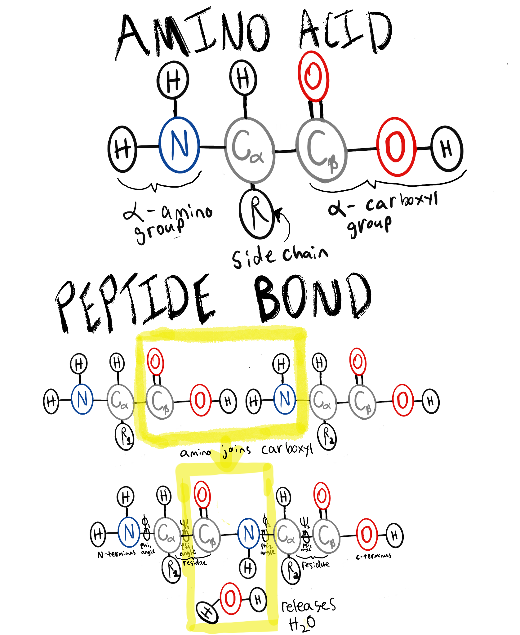
What is a protein? A protein is a chain of amino acids, generally folded into some conformation (shape). Each amino acid consists of an amino group ($N$) and a carboxyl group ($COOH$), a side-chain $R$, and a carbon atom $C_\alpha$ linking them together (see “amino acid” in below figure). The amino group of one amino acid can condense to the carboxyl group of another amino acid, linking the residues together in a polypeptide chain (see “peptide bond” in the below figure). Non-covalent forces such as ionic bonds, hydrophobic interactions, hydrogen bonding, and van der Waals forces act on the residue side-chains, causing these poly-peptide chains to fold into a consistent shape.
What is the protein structure prediction problem? Protein structure prediction determines the folded protein shape from an input amino acid sequence. This consists of coordinates, and rotations, i.e. determining:
- Coordinates for all atoms of all residues in the chain. The atoms of a residue are either:
- Backbone atoms that connect residues together in a chain ($C_\alpha$, pictured above, in the “amino acid” figure).
- Sidechain atoms of a residue vary based on the amino acid type (pictured above, in the “amino acid” figure, as “R”). Sidechains make the amino acid hydrophobic, polar, charged, or have other properties that cause folding forces.1
- Torsion angles of the bonds to $C_\alpha$, $\phi \text{ (phi)}$ and $\psi \text{ (psi)}$, which determine the orientation of the side-chain.2
Predicting a 3D structure from an amino acid string seems like an almost generative task (more like generating an image from a caption than predicting a label for an image). Why should the structure prediction problem be tractable? To quote from the AlphaFold Outputs post:
There are a few points of hope for why in-silico methods could solve for the structures:
The proteins themselves fold in milliseconds, as noted in Levinthal’s paradox. The speed of the folding process hints that some relatively simple rules could guide the overall process, and final folded structure, for biologically useful proteins.
Natural selection favors biologically useful proteins, of which there are far fewer than the theoretical maximum. Natural selection also favors tinkering, so similar structures tend to appear across species.
What information does the AlphaFold system use to predict protein structure? The inputs of the AlphaFold system are:
- An amino acid sequence whose structure should be solved.
- Evolutionarily similar amino acid sequences, in the form of a multiple-sequence alignment (MSA):
- Cluster-level features of each related sequence group (e.g. amino acid sequence of the cluster center, deletions, profile of amino acids within the cluster).
- “Extra” sequence alignments, not selected as a cluster center (e.g. amino acid sequence, mask of deletions and their values).
- Template structure of a few similar amino acid sequences with previously solved structure (e.g. amino acid sequence; pairwise binned distances (“distogram”) among beta carbon atoms; angles of each atom in the residue, and the angle(s) of the sidechain; mask to remove features when the position was unsolved).
The AlphaFold multimer system inputs are similar; each residue position is augmented with a chain ID.
What is the evaluation data for protein structure prediction? Nearly all evaluation data comes from protein structures solved by scientists. Many techniques involve crystallizing a protein, and leveraging the regularity of the crystal structure to solve the structure (e.g. measuring x-ray diffraction strength at different orientations through the crystal). In general, scientists deposit solutions to the protein data bank, uniprot, and other centralized databases for knowledge sharing.
Scientists sometimes advertise in-progress, novel sequences they’re solving through a contest called Critial Assessment of Techniques for Protein Structure Prediction (CASP). In CASP, teams attempt to solve the structures in-silico while the researchers establish the ground-truth in parallel. Once the scientists solve the novel structure, the in-silico submissions are compared to the ground-truth. The most similar in-silico structure is declared the winner. In the CASP-14 contest, the DeepMind team’s solutions from AlphaFold were nearly as accurate as the experimentally determined structures themselves.
What is the training data for AlphaFold? The protein databank contains all of the training data. There were two flavors: solved structures from scientists (which served as ground truth) and unsolved structures where AlphaFold had high confidence (self-distillation set, Supplementary Section 1.3).
What quality metrics are used for evaluation? There are several: global distance test, template-modeling score, and local distance difference test. See the quality metrics section on the AlphaFold Outputs post.
What caveats come with the solved structures in protein structure prediction? Since scientists often crystallize proteins in order to image them at high resolution, the ground-truth structures are neither (1) in situ nor (2) operating dynamically. According to Henzler-Wildman in Dynamic personalities of proteins, there are tradeoffs between local resolution and determining rates of interconversion between stable conformations: highly stable conformations (such as a crystallized protein) provide high resolution, but less kinetic information; while other techniques like NMR can be tuned to have higher kinetic information at lower resolutions. These techniques can be complimentary, since knowledge of the stable structure can provide insights into its fluctuation. For example, fluorescent atomic tracers can track motion of single molecules, and paired with knowledge of the final conformation, one can use these fluorescent probes to determine structural motion on many different timescales.
Other techniques like live-cell imaging can provide a good view of cellular dynamics at several orders of magnitude larger than individual proteins. A single amino acid is roughly 6 atoms wide, on the order of $10^{-9}$m wide, while a cell has width on the order of $10^{-6}$ (see length scales).
Evoformer
What is the Evoformer? The Evoformer jointly updates a representation of pairs of residues of the sequence being folded, with a representation of many, evolutionarily similar sequences. The Evoformer stack consists of 42 Evoformer blocks (pictured below).
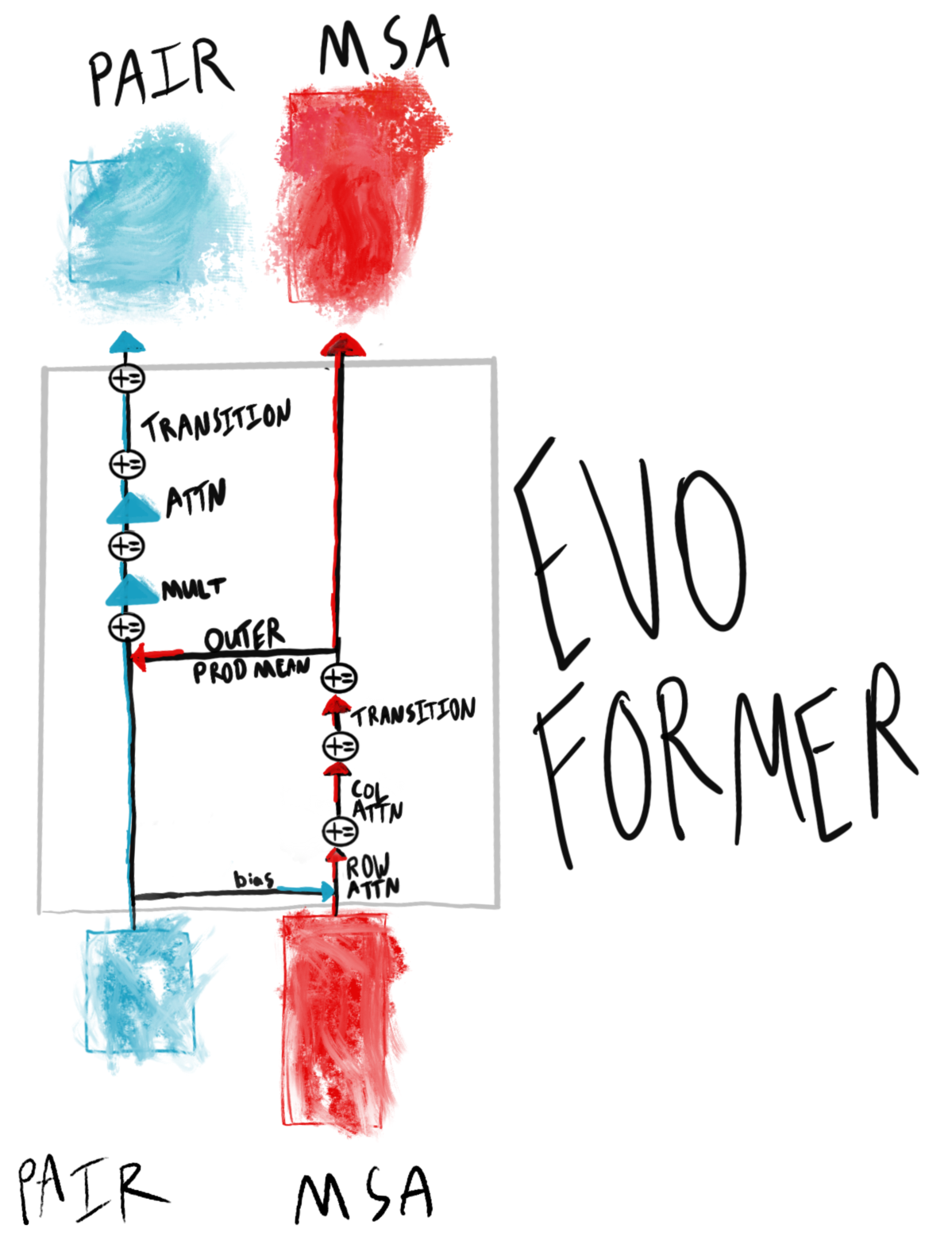
In the Evoformer (Algorithm 6), what are the pair and MSA representations? The pair representation ($N_{res} \times N_{res} \times c$) contains sequence-specific information about how the input residues should interact with each other when folding. The MSA representation ($N_{seq} \times N_{res} \times c$) embeds information about a range of evolutionarily similar sequences for each input residue. Taken together, the two representations can provide novel solutions for a specific sequence via the pair representation, informed with similar, relevant sequences across species via the MSA representation.
As an example, green fluorescent protein may fold quite similarly to fluorescent protein of other colors (e.g. blue, red). The MSA representation can leverage similar structural motifs that cause fluorescence, while the pair representation can account for the specifics that make GFP green.
How does the Evoformer update the MSA representation? The MSA representation is updated first with row-level attention (over each individual MSA profile, Algorithm 7), then with column-level attention (over each position in the alignment to the source sequence, Algorithm 8). The decomposition reduces memory usage.
One other note is the MSA is masked (Supplementary Section 1.2.7), and an auxilary BERT-like loss encourages recovery of the masked values (Supplementary Section 1.9.9). See this post’s Loss section for more information.
How does the Evoformer update the pair representation? The Pair representation is updated via “triangle” operations (Multiplication, Attention). In part, the motivation is that pair representation ultimately informs the structure, and pairwise relations should be symmetrical (e.g. in a triangle, all $ijk$ paths would be the same distance, regardless of permutation). Rather than impose such a hard constraint on the model, however, the triangle updates enable the model to learn this constraint to the extent that it is useful for structure predictions, with two operations:
- Multiplicative triangle updates (Supplementary Section 1.6.5) that use gating from edge $ij$ to incorporate $ik \text{, } kj$ edge product representations.
- Triangle self-attention (Supplementary Section 1.6.6) that updates an $ij$ edge with query-key similarity to the $ik$ edge, and bias term from the $jk$ edge.
What communication is there between the pair and MSA representations? The communication is bidirectional:
- Pair->MSA: the pair representation is projected into a bias term during MSA row (full sequence) attention (Algorithm 7).
- MSA->Pair: the MSA’s outer product mean ($N_{seq} \times N_{res}$) is projected into an update on the pair representation (Algorithm 10).
What is some of the motivation for the “Transition” operations (Algorithms 9 and 15)? Since the transition layers increase, then restore, dimensionality (Algorithms 9 and 15), they may be responsible for some amount of de-noising. Both the MSA and pair representations utilize dropout during their respective updates. It’s possible one function of the transition is to restore some consistency lost due to “dropped-out” row updates.
What are the inputs to the Evoformer? The inputs to the Evoformer are sequence-level features of the protein to be folded, and an MSA representation of evolutionarily similar sequences. At the input layer, the amino acids are embedded into sequence matrices. “Extra” MSAs and template structures are incorporated at the input layer (detailed below).
From each Evoformer layer thereafter, the outputs (pair, MSA) of the prior Evoformer are fed as inputs.
How are the template structures and “extra” MSAs utilized? In addition to MSA cluster profiles (per-position histograms of amino acids within the cluster), a database search component returns sequences with solved structures (“templates”), and individual sequences (“extra MSAs”). This information can prove helpful in solving the structure, and are used in the following way:
- The “extra” MSAs are used in a small (for perhaps compuational reasons), mini-Evoformer (ExtraMSAStack, Algorithm 18) to update the pair representation prior to the first Evoformer block.
- Projections of the template torsion angles are concatenated into the MSA representation.
- Pairwise template representations are added to the pair representation as residual updates.
One suspects two reasons for these relatively simple mechanisms to integrate these extra features:
- The Evoformer is computationally expensive, and therefore it is helpful to reduce dimensionality early on. Reducing the “extra” MSAs into the pair representation incorporates their information without exploding computational complexity.
- The network may become too reliant on template features if the templates are used throughout the network, so incorporating template features only shallowly within the input layer reduces over-fitting.
Structure
What does the structure module do? The structure module generates the folded structure, in the form of atomic positions for each atom in each residue of the sequence, and in torsion angles of the bonds and side-chains.
What are the key representations of the structure module? The structure module consists of three main representations:
- An abstract single representation.
- Backbone reference frames, for each residue.
- The output angles and atomic positions.
(2) consists internally of residue-local reference frames, which are converted to global coordinates as needed.
What sub-modules form the structure module? The key component is the Invariant Point Attention module, which refines the abstract, single-representation with a residual update, based on inputs from the prior single representation, the pair representation (from the Evoformer module), and the backbone reference frames (either the previous structure layer, or identity reference frames during initialization).
The other modules use the single-representation to create a backbone reference frame update for each residue, as well as torsion angles for each residue (which dictate atomic positions).
How does the Invariant Point Attention (IPA) module (Algorithm 22) work, mechanically?
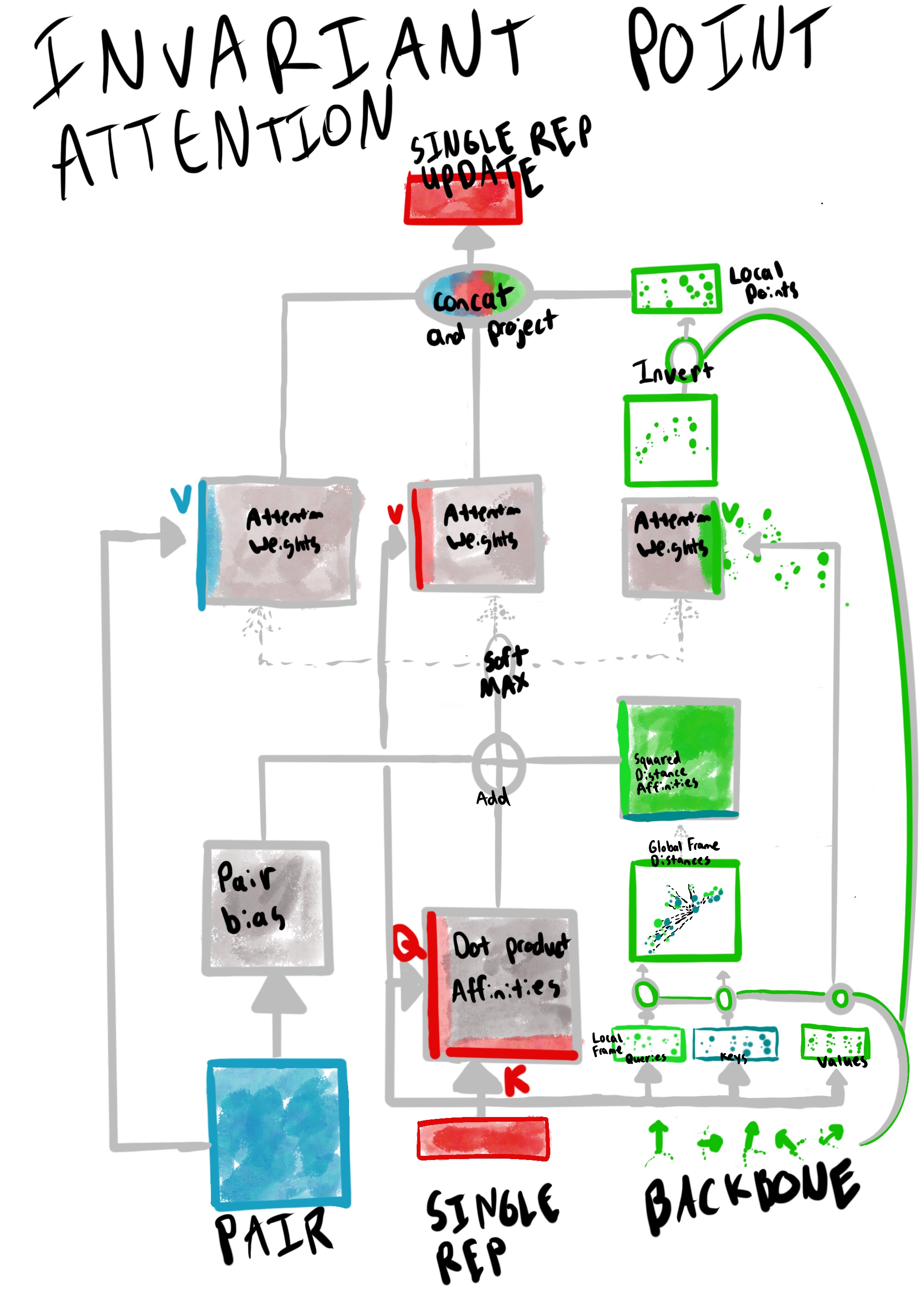
(Figure adapted from Supplementary Figure 8). The Invariant Point Attention module combines signals from the Evoformer’s pair representation, the single representation, and its current set of atomic coordinates for the backbone atoms into an update to its single representation.
The novelty of IPA is in the attention over 3D points. Mechanically, this attention works as follows:
- The point-attention projects the single representation into a few points for each residue to use as query ($\overrightarrow{q_i}$). key ($\overrightarrow{k_i}$), and value ($\overrightarrow{v_i}$) points in residue-local frames. These points are then each projected into a global reference frame (via each residue’s local-to-global reference frame transformation, $T_i$).
- A logits matrix based on pairwise-distance between query points ($\overrightarrow{q_i}$) and key points ($\overrightarrow{k_i}$) in the global frame are combined with logits matrices of single and pair representations to build a joint affinity matrix $a_{ij}$3.
- Value points in the global reference frame ($\overrightarrow{v_i}$) frame are then weighted by the joint affinity matrix $a_{ij}$, and inverted back to their local reference frames (via $T^{-1}_i$).
The single and pair representation attention values are computed relatively similarly: the joint affinity matrix $a_{ij}$ is used to compute the weighted values for each.
Once attention vectors are computed for each representation (single, pair, and point), a final projection layer merges these values into an update for the single representation.
To what does the “invariant” term (of “Invariant Point Attention”) refer? The “invariant” term refers to SE(3) invariance: that is, invariance to global, rigid transformations such as rotation and translation. Sensitivity to such global transformations would explode the state space, so from a modelling perspective, adding SE(3) invariance is highly desirable. According to Supplementary Section 1.8.2, the invariance emerges from the careful handling of points in the global reference frame, and in particular, two places:
- The pairwise-distance affinity matrix calculation (Algorithm 22 L7). Since each point in the pairwise distance computation will be moved identically under a global transformation, the distance matrix computation effectively cancels out any rigid, global transformations.
- Converting the IPA output points in the global frame back into the local frame (Algorithm 22 L10). Any global transformation will also be cancelled out in this conversion back to local frames, since every local frame will invert the global transformation identically.
How do the key components of the structure module interact? The “single representation” gets updated residually using the backbone (via IPA), and the backbone is updated with the single representation. The angles between the bonds are computed separately, from the single representation.
How does the structure module use the Evoformer outputs (Pair, MSA)? First, the initial “single” representation of the structure module is a projection of the Evoformer’s first row of the MSA representation.
Second, the invariant point attention module combines the pair representation, previous single-representation, and points generated along the backbone into a residual update to the single representation.
Can the IPA module inform why the model emits spaghetti-like appendages in the protein domain when it’s uncertain? One particular failure mode for the AlphaFold model is to move low-confidence regions of the residue chain away from the other modules. As an example, take the model’s predictions for GFP structure: while the TM-score is nearly perfect overall, a single low-confidence spaghetti appendage sticks out, away from the overall structure. The predicted SARS-CoV-2 spike protein structure also exhibits similar behavior, although the spaghetti appendage arced along the initial structure (rather than sticking out sideways).
One hypothesis to explain the “spaghetti-ing” is that: patterns the IPA module can’t immediately recognize are shifted “off to the side” as spaghetti strands, to be processed later. There are perhaps two reasons for this behavior:
- Primarily, the distance-dependent affinities will downweight the uncertain portion of the chain significantly. Spaghetti-ing in the IPA module enables progress on the parts of the chain it can tackle, with minimal interference from the spaghetti-ed residues.
- Perhaps a future refinement will yield a solution (e.g. a new iteration of recycling and IPA will yield some new insights).
To support this hypothesis, one can analyze “trajectories” that DeepMind has posted here. The specifics of how the trajectories are created are unclear; one suspects a tool feeds in the pair and MSA representations from the Evoformer to the structure module after each Evoformer block (rather than after the entire stack).
In any case, watch the green and dark blue chains in the earlier frame (42) and in the final frame (153) in the below animation. Notice that the green chain is initially outside, and brought inwards, anti-parallel to the other sheets, while the dark blue chain is initially inside, and eventually “spaghetti-ed” outwards. While it is difficult to make strong conclusions from this single example, one wonders if there is a hint here for how the IPA works with the recycling module (discussed next).

Recycling
What is recycling in the AlphaFold model? Recycling extends a model’s depth by running it $N_{recycle}$ times, passing the predictions (possibly via an embedding) of one iteration of the model (i.e. single representation, pairwise distogram embeddings between backbone alpha carbons) as inputs to the next iteration. At training time, each step computes the loss function after a random number of recycling iterations (between 1 and $N_{recycle}$), which both encourages valid outputs after each recycling iteration and improves computational efficiency.
The name “recycling” evokes some amount of messiness to clean up, before extracting useful information: similar to how a used soda can may contain residual sugars that the recycling process must remove to extract useful metal, it is possible that the network must learn to perform similar “clean up” operations on the embedded outputs when it runs “recycling” iterations.
Further, the metaphor encapsulates the varying degree of cleanup required to attain a useful output when “recycling.” Just as a greasy, cheesy pizza box may be nearly unsalvageable, and a clean glass bottle may be easy to process, the quality of templates/MSAs or first recycling outputs may determine the amount of recycling usage the model requires to fold the protein. Hiqh-quality templates, a large number of MSAs, or a well known sequence may require small, simple tweaks from an initial recycling output, while missing templates or a synthetic sequence may require large amounts of “cleanup” during recycling.
The term “recycling” seems apt, and may become a more generic technique for iterative refinement problems using transformers or resnets.
How is the “recurrent” connection in recycling different from other recurrent neural networks (such as LSTMs)? Mechanically, the self-connection in recycling appears similar to that of recurrent neural networks (such as LSTMs). However, the technique is actually quite different from recurrent neural networks:
- The recycling recurrence serves to increase the depth of the entire model (by a factor of $N_{recycle}$), whereas that of recurrent networks adds/removes relevant sequence information from the node’s hidden state when stepping through the input sequence.
- During training, there is no gradient flow between the recycling iterations, so the modelling is less explicit about the recurrence during backprop than RNN training.
- During recycling, the outputs are embedded (Algorithm 32), rather than used directly (or gated), so one would expect some information loss with this dimensionality change.
- Other inputs (in particular, the MSAs in the input layer) are “re-sample” (Algorithm 2 L5) during each iteration, so recycling also enables further exploration of the inputs. Recurrent networks typically only process the input sequence once.
Both the purposes and mechanics of recurrence differ significantly between Recycling Neural Networks and Recurrent Neural Networks. Recycling is more like Adaptive Computation Time; indeed, one could imagine a network trained to “recycle” until convergence, rather than for a fixed amount of steps.
How is the “parameter sharing” in recycling different from that of convolutional neural networks? Recycling uses an orthogonal parameter sharing mechanism to convolutions. Recycling reuses parameters of a stack of network layers to rerun them on “recycled” inputs, whereas a convolutional layer applies the same parameters for each feature extractor to tiles of the input.
How is recycling different from weight-tying in language modelling? Weight-tying (Press and Wolf) shares an input embedding matrix with the output logits matrix, providing some training signal to all input embeddings (rather than just the one-hot “active” input embedding) at each training step.
In some sense, recycling can be viewed as weight tying, with the following modifications:
- Rather than output-input weights being shared, recycling “shares” the output itself as a new input. By rerunning the whole network stack on this “shared” output, one could think of the network as being effectively “tied”.
- Recycling “shares” the output as the input, by embedding it (Algorithm 32).
One key difference to remember, however, is that at training time, recycling stops gradients between recycling iterations, which lessens the amount of signal transmitted between iterations, as compared to weight-tying.
Why should IPA and Recycling compose so well? Both refine predictions: in fact, the loss functions for the two both encourage incremental success in the structural solution. The structure module computes a light-weight FAPE loss at each layer. Similarly, recycling computes the loss after a random number of iterations (not the maximum number $N_{recycle}$), so each recycling output should improve the structure.
One suspects that recycling enables the IPA module to solve parts of the structure at a time, if needed. In the original AlphaFold paper, Fig 4.b provides examples of recycling convergence for easy and difficult sequences. The latter sequences likely require more exploration of the state space in the IPA module.
Information Flow
What are some design choices of the network architecture that enable information flow? The AlphaFold network consists of many interconnected modules, all of which are trained end-to-end to solve the protein structure prediction problem. As the AlphaFold network is the first to achieve end-to-end neural network to solve the protein structure prediction problem, there must be important architectural choices facilitating proper model convergence. Some architectural choices seem critical to enabling end-to-end training:
- Attention: perhaps the critical motif of the model is attention. Forming outputs from selected points over an entire input sequence enables some form of “deliberation.” Nearly every module in the AlphaFold network utilizes attention in some form (IPA, TriangleSelfAttention, MSA attention, …).
- Residual connections: nearly every portion of the network relies on residual connections, computing incremental updates. Incremental updates have been found helpful for information flow, in ResNets in particular.
- Layer Norm: many modules operate on a LayerNorm-ed copy of their inputs. For example, all Evoformer modules, structure modules, and recycling of the structure into pair distances take the LayerNorm of their inputs prior to using them. It is likely the LayerNorm operation aids in stability of so many end-to-end modules fused together.
- Linear projections: this motif is used so often that one suspects it serves to extract use-case specific information from more general representations. For example, attention relies on projections to generate keys, queries and values from the same inputs (such as the pair, MSA, and single representations). These intermediate representations are often projected to feed auxilary losses, such as the distogram loss. Further, novel components such as triangle attention, IPA, and recycling rely significantly on projections.
Many attention mechanisms (1) are quite novel and ground-breaking. Residual connections, layer norm, and linear projections (2-4) have been relatively common tricks in computer vision since ResNet; with that said, combining these existing techniques with new forms of attention to solve the structure prediction problem likely took deep research and engineering intuition to pull off successfully.
Note that even with all of these motifs, two-pass training is still required for stable convergence, with the second “fine-tuning” pass operating over longer sequences and with more loss terms.
Where in the network is information lost, and, speculatively, why might this information loss be beneficial? Interestingly, there are a number of places information is intentionally lost:
- MSA inputs: different MSA features are used for each recycling iteration.
- Masked MSA: 0.15 of the MSA features are masked.
- Template embedding: the templates are only used in the input layer, a design decision perhaps requiring the model to prefer robust internal representations than attending shallowly to previously solved structures.
- Dropout in Evoformer: both the MSA and pair representations experience high levels of dropout: 0.15 for the former, and 0.25 for each triangle update in the latter.
- Recycling embedder: the 3D structure is reduced to an embedding of pairwise distances during recycling. Angles are not explicitly retained; however, they are likely retained implicitly in the recycling of the single representation.
These steps can be beneficial during training and inference. During training, it is possible that the information removal techniques above may help to “augment” the model’s internal representations, akin data augmentation techniques applied to the input features directly (e.g. filtering, cropping, MSA deletion). At inference time, the model’s noise robustness may reduce overfitting. Recycling in particular seemed helpful in folding SARS-CoV-2 ORF8 protein (fig 4.b), and was relatively important in the ablation study. It’s possible the noise introduced throughout the entire model provides escape from local optima during recycling iterations, thereby forcing the model to explore more of the state space.
What is the “receptive field” of the model? Are there any limitations on which residues can influence a given residue’s position/angles? Overall, the AlphaFold model leverages attention, and therefore is not limited much by receptive field issues like a CNN would be. Additionally, the IPA module attends to structure (not sequence) distance, and any limitations in receptive fields at the structural level are somewhat more likely to map to real physical constraints, rather than model-eccentric limitations.
One main limitation of the model that Al-Quarishi points out is that the cropping during training can influence the maximum-length sequence that AlphaFold may be anticipated to predict correctly. During the fine-tuning phase, the maximum contiguous crop length is 384. However, in addition to his reasons for success (MSA capturing relevant information, full-sequence inference), one wonders if the following also ameliorate the limitation for a single-chain protein:
- Many proteins (such as GFP) would fit entirely within a single crop.
- Large proteins can fold as they are being translated, so the small motifs learned within the crop may account for disproportionate amounts of the structures.
One also suspect the crop limitation makes folding complexes more difficult. The AlphaFold Multimer model upsamples the probability of crops at chain interfaces, so that there’s a 50/50 chance of a training example being an inter-chain crop or an intra-chain crop. While the system works decently well in some conditions, highly complex docking sites may not fit in a cropped sequence length.
Loss
What were the loss functions (Supplementary Section 1.9)? There are a few kinds of losses:
- Structure (FAPE, Aux, distogram)
- MSA mask (BERT loss)
- Confidence (for pLDDT and pTM)
- Violation (fine-tuning only)
What is Frame Aligned Point Error (FAPE, Supplementary Section 1.9.2), and why is it novel? The main parts of FAPE are:
- Frame-Aligned: atoms are scored with respect to their local reference frames. In FAPE, the predicted local reference frame is “aligned” with the ground truth local reference, by simply comparing the relative atom positions directly (and ignoring any difference in the reference frames themselves).
- Point: any number of atom positions of the residue are scored. In the full version of FAPE, all atoms’ positions are compared to the corresponding ground-truth positions; in the alpha-carbon only version, just the alpha carbon position is scored.
- Error: mean clamped squared-distance between analogous atoms in the predicted structure and the ground truth. The error is normalized to be unitless, by a factor of $Z=10$ angstroms. The error term is: $\frac{1}{Z} mean_{i,j}(minimum(d_{clamp}, d_{i,j}))$.
The novelty of FAPE is its:
- invariance to rigid transformation (due to local frames).
- penalization of the incorrect chirality.
What are the other structural losses (besides FAPE)? The “Aux” structure loss scores alpha-carbon FAPE and torsion angle loss, and is computed on each layer of the structure module. FAPE is mentioned above; torsion angle loss is computed by the L2 distance of the predicted and actual unit vectors on the unit circle.
The distogram loss compares a ground-truth distogram with a predicted distogram based on the pair representation, to ensure the pair representation is structurally useful. The distogram loss is binned roughly to the accuracy of 0.3 angstroms.
What is the Masked MSA loss? The Masked MSA loss provides a BERT-like task to reconstruct masked values in the MSA input, encouraging context in the MSA representation. The masked MSA loss was critical in the ablation study (Supplementary Figure 10), suggesting that such protein language modeling over evolutionarily common sequences could embed significant structural relationship. In fact, other research supports the benefits of protein language modeling that leverages evolutionary information: Facebook AI’s ESM approach was moderately successful (and state-of-the-art) in unsupervised contact prediction.
This post’s MSA features has more examples MSAs, and the procedures one might take to generate them.
What are the model-confidence losses? The AlphaFold model predicts per-residue confidences for template-modelling and lDDT. These losses are weighted relatively low, and are primarily used to determine the degree of accuracy for the AlphaFold outputs without supervision.
What is the violation loss? The violation loss penalizes invalid chemical structures, such as bond-lengths and bond-angles that differ from literature values. It also includes a penalty for non-bonded atoms that are closer than their van der Waals radii would allow theoretically.
In some sense, the model can “reason about physics” due to the violation loss. The violation loss term is optimized during fine-tuning, and not on the first-pass of training.
The model is “physics-aware” due to the violation loss - does it ever violate physical constraints with its structure predictions? If so, how does the system correct such invalid structures? As a final post-processing step, the AlphaFold system runs a “relaxer” (“Amber relaxation,” Supplementary Section 1.8.6). The relaxer makes small tweaks to any structural elements violating such constraints. Sometimes, if the relaxer cannot converge, the model is rerun in an attempt to generate a more physically realistic structure.
How does the loss change for the multimer use-case? In the multimer system, FAPE is unclamped at interface boundaries (Section 2.4 in AlphaFold Multimer paper). Further, a greedy search attempts to match chains (which can come from identical sequences) prior to scoring (section 2.1 of the same paper).
MSA Features
This section provides more details on the evolutionarily similar sequences.
What defines an “evolutionarily similar” amino acid sequence to the input sequence (to be folded)? Large protein databases contain proteins from many species. Some of these proteins, called homologs, are related structurally. Although homologous proteins can differ significantly in amino acid sequence, often, two proteins with high sequence similarity will also have homologous structure. For example, the delta variant of SARS-CoV-2 spike protein differs from the original by just a few mutations in a thousand-long aa sequence4. Therefore, information about the structure of the original spike protein would yield tremendous insight into the structure of the (sequentially similar) delta spike protein. The pattern tends to hold for less extreme examples, as well.
What is the search procedure for finding “evolutionarily similar” sequences, and what quality metrics determine its success? First, finding such homologous sequences will use profile HMMs. While there are a variety of such procedures, the search procedure for JackHMMER is as follows:
- From an initial query sequence, find similar sequences with low BLAST E-value.
- From these similar sequences, construct a profile HMM.
- Use the profile HMM to score a large database of sequences. Align the most likely sequences, and update the profile HMM with these alignments.
- Repeat (3) until either no new sequences are returned, or some maximum number of iterations is reached. Note: since (3) is run on large datasets, iteratively, there are some optimizations (HMMERHEAD tiered-filtering: “word”-level filtering, multi-word filtering, then full Viterbi filtering).
In general, such search procedures are evaluated on sensitivity and specificity:
- Sensitivity is measured with structurally similar homologs (e.g. the SCOP database categorizations). Since the associations are based on structure, the sequences may vary somewhat. It is assumed that similar amino acid sequences will form similar structures; however, it is not assumed that proteins of similar structure would have similar amino acid sequences.
- Specificity is determined by a distracting set. In some cases, this set consists of the “positive” set, but with the sequences randomly shuffled.
By tuning sensitivity on proteins with homologous structure, the search procedure will tend to return some proteins of similar structure.
Training Setup
What training set was used? Datasets of up to 150k sequences from the protein databank and 350k sequences from the self-distillation dataset are sampled at proportions of 25% and 75%, respectively, during training.
The model trains for 7.5M samples (combining initial and fine-tuning), giving ~80k mini-batches of size 128. Therefore, each sequence would be sampled approximately 21 times, in expectation.
Approximately how much time (on average) does a single training batch (fwd+bwd passes) take? With a mini-batch size of 128 (Supplementary Section 1.11.3), on a 128-TPU pod,
- Initial training takes ~10s per batch. 6M sequences would fit into ~46k mini-batches. If it takes about 1 week to complete these batches, on average, 4.7 batches can be completed in a minute (about 10s per batch).
- Fine tuning takes ~60s per batch. 1.5M sequences would fit into ~11k mini-batches. If it took 4 days to complete these batches, on average, about 1.1 batches can be completed in a minute (about 60s per batch).
What’s an estimate of the computing cost to train a single AlphaFold model? Speculatively, $\$33k$ to run a V3-128 TPU pod for 11 days (7 days initially with 4 days of fine-tuning), at evaluation pricing, assuming the pricing for a V3 128-TPU pod is 33% more expensive than v2-equivalent (as the v3 32-TPU pod is compared to the v2 32-TPU pod). However, this pricing quote is speculative since the V3 128-TPU pod’s price is unspecified, and the best way to get the “real” number would be to contact the Google sales department.
Inference
How big is an AlphaFold model? The model is 93M params (txt tabulation)5.
- Most parameters are dedicated to the Evoformer (~91M), split among MSA layers (~64M), pair layers (~24M), and input processing.
- The rest are used in the structure module (~2M) and additional output heads (~100k).
In total, the AlphaFold model uses 371MB of disk space. As a reference, the GPT-2 is 237MB in float16 TFLite format.
Why is the AlphaFold model expensive to run, as the sequence length increases? AlphaFold runs on the full, un-cropped sequence. Accordingly, the Evoformer module cost grows with the sequence length: Triangle-related updates (TriangleSelfAttention, TriangleMultiplication) require $O(N_{res}^3)$ computations, and the MSA attention computation cost grows with $O(N_{seq} \times N_{res})$.
What’s more, these costs also multiply by 20 running the full pipeline:
- Recycling runs each model 4 times to solve for an input structure.
- The AlphaFold pipeline runs 5 separate models, to select the highest confidence structure as output.
Sources
The detailed supplementary information for AlphaFold has in-depth information on each component of the AlphaFold system. I mirrored the snapshot I looked at on my own site here.
Mohammed Al-Quraishi’s blog post on the method paper provided insights into some AlphaFold design decisions that uniquely tackle the protein structure prediction problem. His overview of the implications of AlphaFold is also worth a read to help put the problem into context.
This detailed post by Justas Dauparas and Fabian Fuchs also does a good job explaining the background. I found their in-depth overview of the concept of an SE(3) transformer helpful.
proteinstructures.org provides helpful context on protein structure terminology, modeling, and more.
Acknowledgements
Thanks to June (Yuan) Shangguan for providing feedback on earlier drafts of this post.
proteinstructures.com gives a good overview of amino acids, and their relevant properties to protein folding. ↩︎
proteinstructures.com provides more detail on torsion angles, and their effects on the folded structure. ↩︎
“Affinity matrix” performs the softmax operation on the logits matrix in the attention. ↩︎
See a visualization of the spike protein here. The delta variant spike protein visualization is near the bottom of the page. ↩︎
My first attempts at profiling the JAX model with TensorBoard failed for various reasons. Future updates to this post may include a more complete “profiling AlphaFold” section, after some of the bugs are worked out. In the meantime, the
haiku.experimental.tabulatefunction dumped per-module parameter usage (without any runtime information): see here ↩︎